
Capacity Planning
Definition- Determining the production schedule needed to meet changing demands for products. You’ve got stuff to make. How do you figure out how much to make, and when? Capacity Planning. It can take many forms. There is lot-for-lot, fixed order quantity, fixed order period, and a less well known option of part-period balancing.
Before we dive into them all, we gotta know about the Wagner-Whitin Property.*
“Under an optimal lot-sizing policy either the inventory carried to period t +1 from a previous period will be zero or the production quantity in period t + 1 will be zero.”
Basically, it never makes sense to produce what’s needed in a single period over a spread of multiple periods. Other assumptions baked in are that demand and production are deterministic. Uncertainties such as canceled orders, mechanical breakdowns, sickness, etc. are not baked in. With that in mind, let’s look at some options for capacity planning.
Let’s start with a fictional demand schedule:
| Time period | 1 | 2 | 3 | 4 | 5 | 6 | 7 | 8 |
| Net Requirements | 12 | 15 | 60 | 24 | 48 | 21 | 61 | 29 |
For simplicity, we can think of each time period as a week, and the net requirements as generic “units.” Could be shoes, monitors, desks, or anything.
In Lot-for-lot planning, one would simply make the number of parts needed in the period they are needed in. So, for period one, you would make 12 units, period two make 15 units, period three make 60 units, etc. This method minimizes inventory because nothing is ever carried forward. It’s the simplest form of capacity planning. When set up costs are minimal, this approach makes a lot of sense, assuming you have the capacity to produce the requirements in a given period. If you do not have the capacity to produce all the demanded units in a particular time period, you’ll need to take a different approach.
In Fixed Order Quantity, one determines a fixed number of items to produce at a time. Reasons being, you might have a certain size of transportation equipment in your facility, meaning it makes sense to produce a fixed amount that can easily be moved. Or, by finding a particular order size you can cut down on the number of set ups required. Finding the order quantity is done with the following equation;
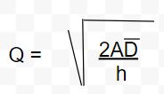
Where Q = the order quantity, A = the set up costs associated with producing the item(s), D = average demand, and h = inventory carrying cost per unit per period. For simplicity, we’re ignoring interest rates here. Rigidly following this method likely means you’re not meeting the Wagner-Whitin property. You’ll carry inventory from one period to another, and only make more units as needed. In most cases, you would end up producing the units needed for one period in multiple periods (you don’t want to do that). The other downside is that you end up with excessive inventory, thus a carrying cost, and you still need to incur set up costs. To get around this, you can determine your Quantity (Q), and adjust it to be closest to the exact demand of one or more periods.
Example: If we found that, in this scenario, the optimal Q = 85 units, using the above demand schedule, the production schedule might look like;
| Time period | 1 | 2 | 3 | 4 | 5 | 6 | 7 | 8 |
| Net Requirements | 12 | 15 | 60 | 24 | 48 | 21 | 61 | 29 |
| Items made | 27 | 84 | 69 | 61 | 29 |
Without regarding the Wagner-Whitin property, the schedule would look like this;
| Time period | 1 | 2 | 3 | 4 | 5 | 6 | 7 | 8 |
| Net Requirements | 12 | 15 | 60 | 24 | 48 | 21 | 61 | 29 |
| Items made | 85 | 0 | 85 | 0 | 0 | 85 | 0 | 85 |
| inventory | 85-12=73 | 73-15=58 | 58+85-60 = 83 | 83-24= 59 | 59-48= 11 | 11+85-21= 75 | 75-61= 14 | 14+85-29= 70 |
Failing to take into account the Wagner-Whitin Property means you end up producing units for period 3 in both periods 1 and 3. And, because of a limit in how far out we see demand, you end up with 70 units that may go bad. Not ideal, but given your circumstances this method might make sense if set up costs need to be minimized, demand is steady, and holding costs are low.
In Fixed Order Period, one follows a similar approach to above, but instead of optimizing for a particular interval size, one optimizes for a particular frequency of ordering. The optimal order period can be derived by taking Q, calculated above, and dividing by average demand per period. Assuming Q= 85, and average demand equals 33.75 (sum of Net requirements divided by number of time periods), then the orders should be placed every;
P = Q/D
P = 85 / 33.75
P = 2.52
P~= 3
That manufacturing schedule would look like;
| Time period | 1 | 2 | 3 | 4 | 5 | 6 | 7 | 8 |
| Net Requirements | 12 | 15 | 60 | 24 | 48 | 21 | 61 | 29 |
| Items made | 87 | 93 | 90 |
This meets the Wagner-Whitin Property because it never makes units for one period over the course of multiple periods. It does carry inventory forward, but only in quantities that correspond to exact demand (this is why we assumed demand to be deterministic at the beginning). One nuance to this approach that should be touched on is that in a period of zero demand, no items will be made, even if the order interval otherwise says to produce. In the above table, for example, if period one had a demand of zero, nothing would be made until period two when there is a demand of 15. Future production runs would then be offset by periods that have no demand.
Finally, Part-Period Balancing (PPB). This method combines the Wagner-Whitin property with the assumption that inventory carrying cost is equal to the setup cost. The motivation for using PPB approach is to balance the inventory carrying costs and the setup costs so neither one blows up. A part-period is the length of time a part is carried. E.g. 1 part carried for 10 periods, 5 parts carries for 2 periods, and 10 parts carried for 1 period all are 10 part-periods and have the same inventory carrying cost. Let’s see an example.
For this scenario, let’s assume the setup cost is $200 (constant) and the carrying cost is $2 per item per period. The demand schedule will remain the same as above.
| Quantity for Period 1 | Setup Cost ($) | Part-Periods | Inventory Carrying Cost ($) |
| 12 | $200 | 0 | 0 |
| 27 | $200 | 15 * 1 = 15 | 15*2 = $30 |
| 87 | $200 | 15+60 * 2 = 135 | 135 *2 = $270 |
| 111 | $200 | 135 + 24*3 = 207 | 207* 2 = $414 |
Since $270 is closest to $200, you would choose to build 87 items in period 1. That would cover the needs for periods 1, 2 and 3. Doing it again-
| Quantity for Period 4 | Setup Cost ($) | Part-Periods | Inventory Carrying Cost ($) |
| 24 | $200 | 0 | 0 |
| 72 | $200 | 48*1 = 48 | 48 *2 = $96 |
| 93 | $200 | 48 + 21*2 = 90 | 90 *2 = $180 |
| 153 | $200 | 90 + 61*3 = 273 | 273 * 2 = $546 |
Now we can see that $180 is closest to $200, so we’ll build 93 items. This will cover periods 4,5 and 6. Again, we go!
| Quantity for Period 7 | Setup Cost ($) | Part-Periods | Inventory Carrying Cost ($) |
| 61 | $200 | 0 | 0 |
| 90 | $200 | 29 *1 = 29 | 29*2 = $58 |
Since we don’t have a planning horizon beyond 8 weeks here, we would stop. In week 7 we would choose to build 90 units to cover periods 7 and 8. The actual schedule would look like this;
| Time period | 1 | 2 | 3 | 4 | 5 | 6 | 7 | 8 |
| Items made | 87 | 93 | 90 |
Note, this is the same schedule as the Fixed Order Period.
Where is this used?
- Manufacturing
- Packaging
- Long term business planning
- Software infrastructure
- Budgeting
When it comes to making stuff, spending the time figuring out how much to make and when will set you up for a much smoother operation. It makes scheduling a work force easier. It makes responding to new orders easier since you know exactly when you can get to a new order. Regardless of what you’re producing, having a schedule for it will bring better results than making everything ad hoc.
*Hopp, Wallace J., Factory Physics Second Edition, (2000)
