
Linear programming is a mathematical technique for finding optimal solutions to linear equations. Generally used to solve for maximizing profits or lowering costs) Basically, when there are multiple options on the table governed by linear equations and linear constraints, linear programming is how to find the best option.
In simple cases with only two variables, the system of equations can be solved graphically, which is pretty cool. Below is an example of a simple linear program with only two variables.
A simple case, courtesy of Wayne Winston.
A woodworking shop wants to maximize weekly profits. It makes two products, a soldier, and a wooden train. A soldier sells for $27, and has $10 of raw material inputs. The work involved adds $14 of variable overhead. A train sells for $21, uses $9 of raw material, and adds $10 of variable overhead. A soldier requires 2 hours of finishing work, and one hour of carpentry. A train requires one hour of finishing and one hour of carpentry. Each week there are 100 hours of finishing, and 80 hours of carpentry labor available. Demand for the train is unlimited, but only 40 soldiers sell each week.
What is the optimal workload to maximize profits?
| Item | revenue | Raw material cost | Variable labor cost | Carpentry work (max 80) | Finishing work (max 100) |
| Soldier (x1) | $27 | $10 | $14 | 1 hour | 2 hours |
| Train (x2) | $21 | $9 | $10 | 1 hour | 1 hour |
Weekly revenue = weekly revenue of soldiers + weekly revenue of trains
Weekly profits = weekly revenue – weekly costs
Weekly raw material costs = 10x1 + 9x2
Weekly variable costs = 14x1 + 10x2
(Assuming fixed costs don’t matter for the example)
So we want to maximize;
(27x1 + 21x2) – (10x1 + 9x2) – (14x1 + 10x2) = 3×1 + 2x2 = z
Constraints-
Carpentry; x1 + x2 <= 80 hours (blue line below)
Finishing; 2x1 + x2 <= 100 hours (purple line below)
Demand constraint; x1 <= 40
*Assume raw material has no constraint.
Sign restrictions (neither product can be negative); x1, x2 >= 0
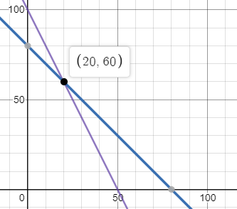
Graph 1: Labor constraints for making trains and soldiers.
This hastily made graph is the two primary constraints (finishing and carpentry labor). Their cross section (20,60) is the optimal solution for maximizing weekly revenue.
So, z = 3x1 + 2x2 = 3(20) + 2(60) = $180
This solution meets all the constraints above, and will produce the highest revenue for the wood shop. (do note, this example assumes the true cost of material and labor to be known with certainty).
Similar math, but more complex than just two variables, can be done in many places to maximize profits, or minimize costs. Examples being a restaurant, bar, hair salon, auto shop, or cafe. In each case there is a menu of options to choose from, each choice coming with a certain cost associated with it (labor input and material input). Solving complex linear programs can be a pain, but thankfully there is software that does it for us now. If you’re in need, LINDO is a free, simple to use tool for solving Linear Programs.
